Etendue and Optical Invariants

By Olov von Hofsten and Simon Olin |

“The possibilities of optics are endless” – you may have heard things like this and it sounds great and wonderful. Unfortunately it is not true – you have been told a lie. The possibilities of optics are NOT endless. In fact, it is very important to know where these limits are. Trying to break the laws of physics is a great way of wasting your time. Trust me.

Smart people have already paved the way here and defined limits. For example, defined things that cannot change: optical invariants. An invariant is something that is constant as other things change in the system. Consider a spherical cow in perfect vacuum (see figure 1). During the size transformer, the cow stays spherical – it is an invariant.

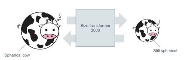
Figure 1. The cow stays spherical during the transformation – it is an invariant.

Optical invariants are important because they show what is physically possible to achieve when dealing with illumination and imaging. There are four main optical invariants:
1. The Lagrange Invariant or the Optical Invariant
2. The Abbe sine condition
3. The Straubel invariant
4. Etendue

These four invariants have different applications and are valid under certain conditions. We will discuss number 1, 2 and 4 in this article.

Let’s start with the Lagrange invariant. Assuming a lossless, paraxial system, this invariant is constant under refraction and is valid between any planes in an optical system. It is defined by the position and angle of the chief and marginal rays. Let’s look at figure 2.

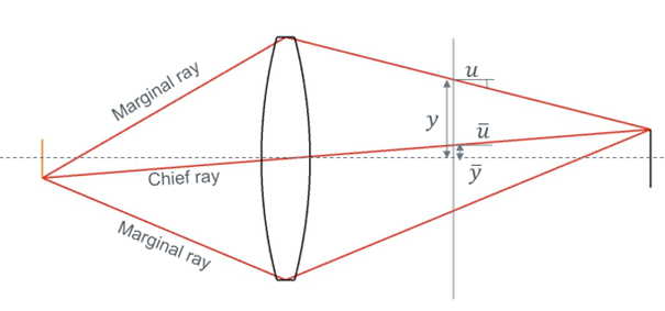
Figure 2. Definition of the entities included in the Lagrange Invariant.

The definition states that the product of the chief ray angle (u-bar) and the marginal ray height minus the product of the marginal ray angle and the chief ray height is constant. Or mathematically:

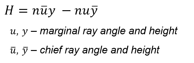
H is the Lagrange Invariant and it remains constant. n is the refractive index. For example, if the marginal ray angle decreases – then either the chief ray height must increase to compensate, or either the chief ray angle or marginal ray height decreases. Consider three places in the ray diagram below for yourself and think about what entities are changing.

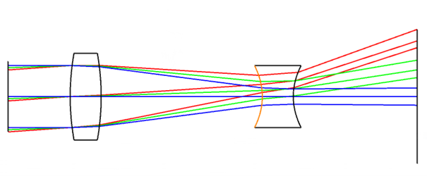
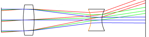
Figure 3. An optical system. Consider rays of the same color. Before the first lens, the marginal ray angle is small and the chief ray height and marginal ray height change in parallel (the light is collimated). The light hits the lens and the for the invariant to remain constant, the angles decrease as the index is increased. After the lens, the angles have increased and the heights change in different directions. After the second lens the light is again collimated so the chief and marginal angle are equal – but larger than before. Therefore the difference in height between the chief ray and the marginal ray is smaller.

All in all, we see that a larger difference in angle means a smaller difference in position, between the marginal and chief ray.

The Optical Invariant is a generalization where the relation is defined as between two arbitrary rays. Which is easy to understand. We could have picked another ray than the marginal ray.

The Abbe sine condition takes the sine(angle) so this is applicable to not only paraxial optics. It is written as

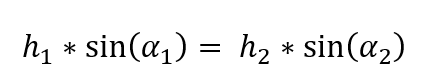
Ernst Abbe developed this invariant for aberration-free (spherical and coma) microscope systems. It is not applicabe to all planes, but between two image planes. h₁ is the maximum ray height in one plane and α₁is the ray angle. And equivalently for another plane, where h₂ is the height and α₂ is the ray angle.

This means that the product of angle space and positions remain constant, when there is no aberrations or losses.

One result of these invariants is that you cannot have any FOV and exit pupil size for a given sensor. H will be constant between the sensor plane and the exit pupil so the same rules apply here. The angles out from the exit pupil will define the FOV and the angles out from the sensor is the F#. Which usually is not lower than 1. See Olov previous blogg post on this!

Now Etendue is like the Abbe sine condition applied to non-imaging systems. In fact, you can see it as H² (since we need to consider two dimensions). You can consider it as area * Solid angle. Let’s looks at a surface of area S, and light emitted at solid angle α:

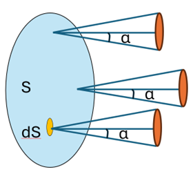
Figure 4. Definition of variables for the etendue

The Etendue is then:

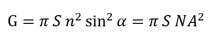
In non-imaging systems we can have things like diffusers, and light can be mixed in different directions and areas since we are not imaging anything. This means that H, or the etendue, can increase. BUT, we cannot decrease it. Well you can – but then you will have losses. This is why the definition says that Etendue can not decrease in a lossless system.

Let’s consider a simple example, the system in figure 4.

For the source we have,

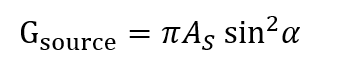
At the lens we have

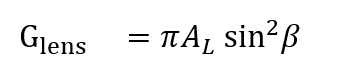
Due to the conservation of Etendue we have (in the absence of losses or diffusors)

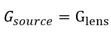
And therefore since

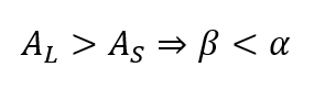
The larger we make A_L, the smaller we can make β. But we also need to make the focal length longer in order to Also note that, if we replace the lens with a diffusor:

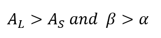
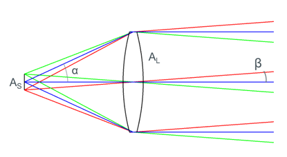
Figure 4. A system with a source and a collimating lens

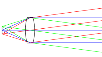
Figure 5. A smaller lens that collects the same amount of light as the lens in figure 4, but the same source size will result in a wider angular spread after the lens.

In a way, the optical invariants bring order to optics deign and we should be happy that we have them. But, as my colleague Gustav often says “Etendue is a b*tch”.