LiDAR Linkbudget

By Olov von Hofsten|

One of the most important specifications of a LiDAR is the range. How far can the LiDAR see? This may be the first question one asks. You quickly realize that this depends on a multitude of extrinsic and intrinsic parameters. For the extrinsic parameters, target reflectivity and sunlight illuminance are the two most important factors (which is why they are usually provided in a spec) but directionality of the surface reflection and albedo, together with the tilt of the surface in reference to the laser beam direction is also highly influential (most cases assume Lambertian surface and normal incidence). There are many intrinsic parameters: Laser beam power, collecting aperture, detector size and filter bandpass. In this post I will try to sort out these parameters and present them in an interactive graph. This work is usually referred to as the link budget since we are trying to calculate the number of photons. We will see that both signal photons and noise photons need to be calculated. In practice, one needs to consider things like the occurrence of negative positives and how sure you want to be on your range. Since that discussion is outside the scope of this article, I set a very hard limit.

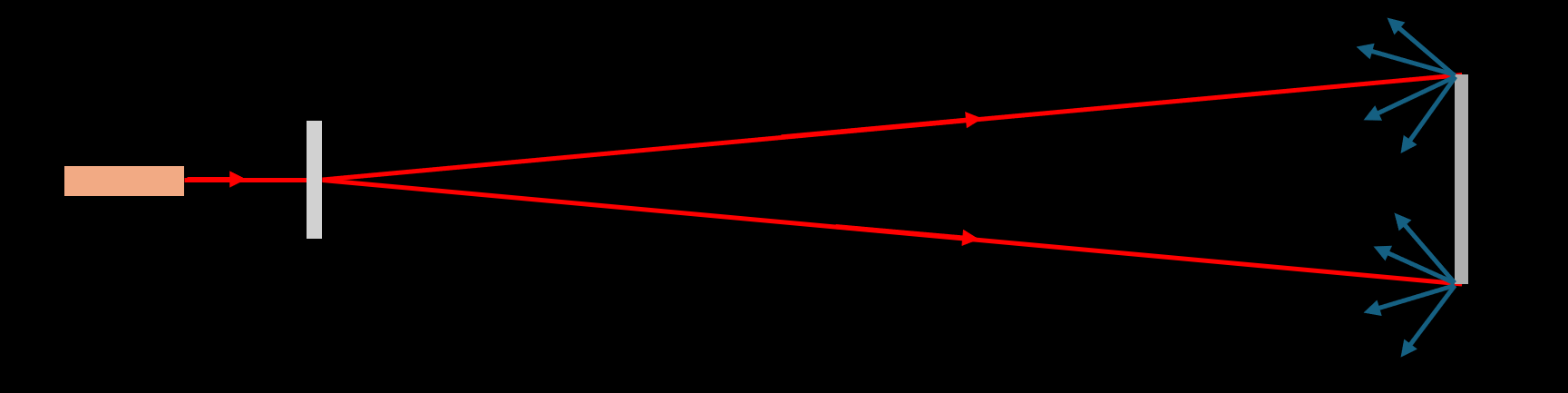
I will only look at time-of-flight flash LiDAR in this blog post. In Fig 1 you can see the setup of a flash LiDAR.

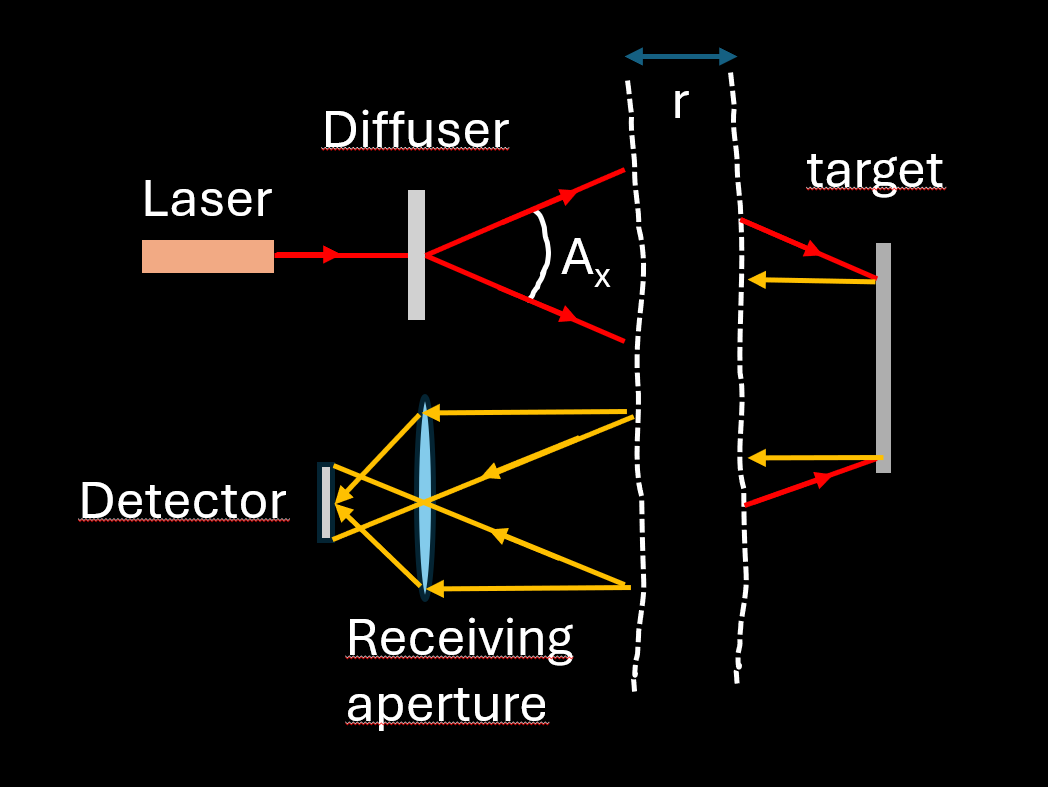
Fig 1. The principle of a Flash Lidar. A laser hits a diffuser which illuminates the entire field-of-view. The light hits a target at a distance r, and light is reflected back to the detector via a receiving aperture.

Emitter

Let’s start with the source of the light. We need a laser. The laser should not be visible to the eye, and it should not be absorbed by water. In addition, we should be able to detect it with standard silicon detectors. This narrow it down to ~900 – 1100 nm. There are three laser wavelengths being widely manufactured in this range: 910, 940 and 1064 nm. These are the wavelengths used in most ToF LiDARs.

When setting the power of the laser we need to consider eye safety. This can get complicated for scanning LiDARs but it is easier in our case with a flash. Assuming a small virtual source (C6 = 1) and the case of the unaided eye, we can use the default (simplified) evaluation with condition 3 (IEC 60825-1:2014, table 10) which yields the following limits for a class 1M laser product for the three listed wavelengths above (ibid, table 3 and table 9)

Wavelength	Accessible emission limit in 7 mm aperture, 100 mm from the LiDAR, for t >10s, Φavg	Pulse energy limit for pulse group (see table 2 and 3 of IEC-60825) for 7 mm aperture, Qmax
910 nm	1.0 mW	195 nJ
940 nm	1.26 mW	225 nJ
1064 nm	1.95 mW	758 nJ*

Table 1: Class 1 eye safety limits assuming C6 = 1, unaided eye. Note that t is the measurement time. *for 1064 nm the pulse group time is 13 µs instead of 5 µs for 910 and 940 nm.

We need to consider both long and short integration time limits (they correspond to two different types of damage to the eye – burning and heating). These are shown in the two columns.

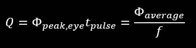
We can start with the average power, when t>10s. With a given laser repetition rate, f, we have the peak pulse power by:

For example, for a 910 nm wavelength, 5 ns pulse time and 2 kHz repetition rate, we need to keep the peak pulse power below 100 W ([HK1] [Ov2] using the values in Table 1, this is valid into a 7 mm aperture at 100 mm distance from the emitting aperture) in order to keep below the longterm limit. For the short time limit we calculate the pulse energy by

For a 100 W peak power and 2 kHz repetition rate, the pulse energy is 500 nJ. This is more than a factor of 2 above the single pulse limit (table 1). We need to increase the laser frequency so that the pulse energy is lower, for a given average power. The minimum frequency allowed is given by

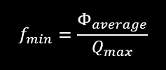
So, we need to increase the repetition frequency to above 5.1 kHz to stay eye safe in the single pulse case.

Next thing to consider is the divergence of the emitter. This will be the area over which the light is spread out, or equally the field-of-view of the flash LiDAR. Let A_X be the horizontal field-of-view of the emitted pulse, and A_y be the vertical field-of-view.

The 7 mm pupil of the eye takes up 4 degrees (we will call this constant α_eye) so with A_x x A_y degrees field-of-view, we have a relation to the emitted peak power by

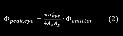
By combining equation (1) and (2) we have

Now switching to f_min for the laser frequency. The emitted peak power is calculated from the efficiency of the emitter, n_emitter and the laser peak power, Φ_laser

Target

So now the light has been emitted and is travelling through space. For long distances, some light will be absorbed in the air. This is wavelength dependent and weather dependent, but a reasonable approximation for our wavelength range is (ref 1)

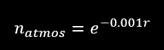
Where r is the distance travelled. The beam hits the target and is reflected. Most link budgets assume a Lambertian target and so will I. Therefore, the solid angle that the light spreads into is simply π. The radiant intensity of the laser beam from the target is therefore

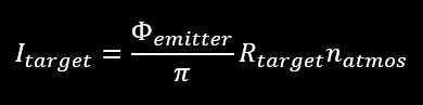
Where R_target  is the target reflectivity.

Receiver

On the way back to the receiver (assuming it is in about the same place as the emitter) light is again absorbed by the air. The amount of light at the receiver is the target radiant intensity multiplied by the receiver solid angle and the absorption factor n_atmos:

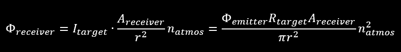
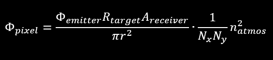
A_receiver is the area of the receiving aperture. If the receiver array is matched to the emitted field, this will be the total received power. Given a certain vertical and horizontal resolution N_x x N_y, the peak power per pixel is

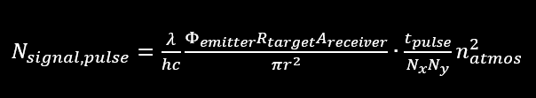
Now we just want to convert this to photons, so therefore we need to multiply by the pulse time and by λ/hc (wavelength divided by Plancks constant and the speed of light, ie the photon energy):

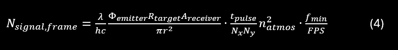
This is the number of photons per pulse. To convert this to photons per frame, we multiply with the repetition rate and divide by the framerate. So finally,

Where FPS is the framerate. So, how many photons do we need? As you may know that is the wrong question. What we want to know is what SNR do we need! This depends on a lot of things and a lot of theory has gone into this. My answer is simple: 17 dB.

To calculate the SNR we need the noise. And in the LiDAR case the source of noise is a big adversary – namely the sun. The sun irradiance on a target depends on the wavelength band you are looking at. The width of the wavelength band depends on how wide you can have your filter on the receiver. Many factors may weigh in on that like temperature range, angles, batch variations…. Fig 2 shows the sun irradiance at sea level with the relevant bands in table 2 highlighted.

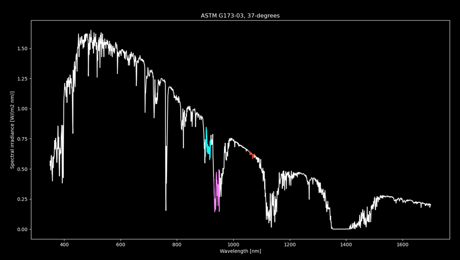
Fig 2. Sun spectrum at sea level according to ASTM G173. 20 nm bands around 910 nm, 940 nm and 1064 nm are shown in cyan, magenta and red respectively.

The 940 nm band contains less sunlight than the 910 nm band due to the H₂O absorption in the atmosphere. Silicon photodiode responsivity is a little bit higher for 940 nm (and lower for 1064 nm) but since I will only be considering optical SNR in this article, I am not taking this into account.

Integrating the data shown in Fig 2 over two different bands give irradiance levels at the target as

Wavelength	Irradiance for 20 nm band, Esun	Irrandiance for 40 nm band, Esun
910 nm	13.7 W/m2	28.5 W/m2
940 nm	6.1 W/m2	16.5 W/m2
1064 nm	12.5 W/m2	25 W/m2

Table 2: Solar irradiance levels for different wavelength bands

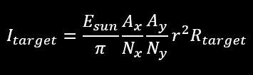
The total number of solar photons on the detector can be calculated from these numbers by multiplying with the footprint of the detector. We start by deriving the radiant intensity by doing this and dividing by pi, plus adding the surface reflectivity:

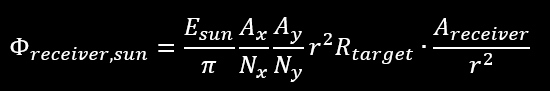
Next step is to multiply by the solid angle of the detector to get the power at the receiver:

It should come to no surprise that the range dependency cancels out (luminance is not distance dependent) and we are left with (simultaneously switching to N_{sun, frame} here, please keep up):

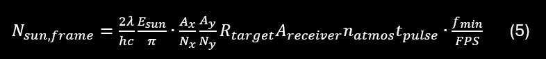
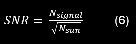
Where I choose 2*t_pulse as the integration time, since the integration time is longer than the pulse time. But this can be discussed. The optical SNR is given by (ref 2)

Here I could of course try and combine equations (3), (4), (5) and (6). But I doubt it would give a better overview. Instead, I have implemented these equations into an online graphing calculator.

https://www.desmos.com/calculator/bqgkvj7iu8?lang=sv-SE

Several conclusions can be drawn from the Desmos calculator. One is that it is better to concentrate light into a short period of time. Longer pulse times lead to lower SNR at the same time. This is what makes dToF LiDAR performing better than iToF, which uses longer pulse/integration times.

A comparison for the three different wavelengths are shown in Fig 3. Clearly, 1064 nm gives the best range of the three due to the higher eye safety limit. But, other things will impact, especially Si PD responsivity. The SNR limit of 17 dB is shown as the red line, but should not be taken as absolute.

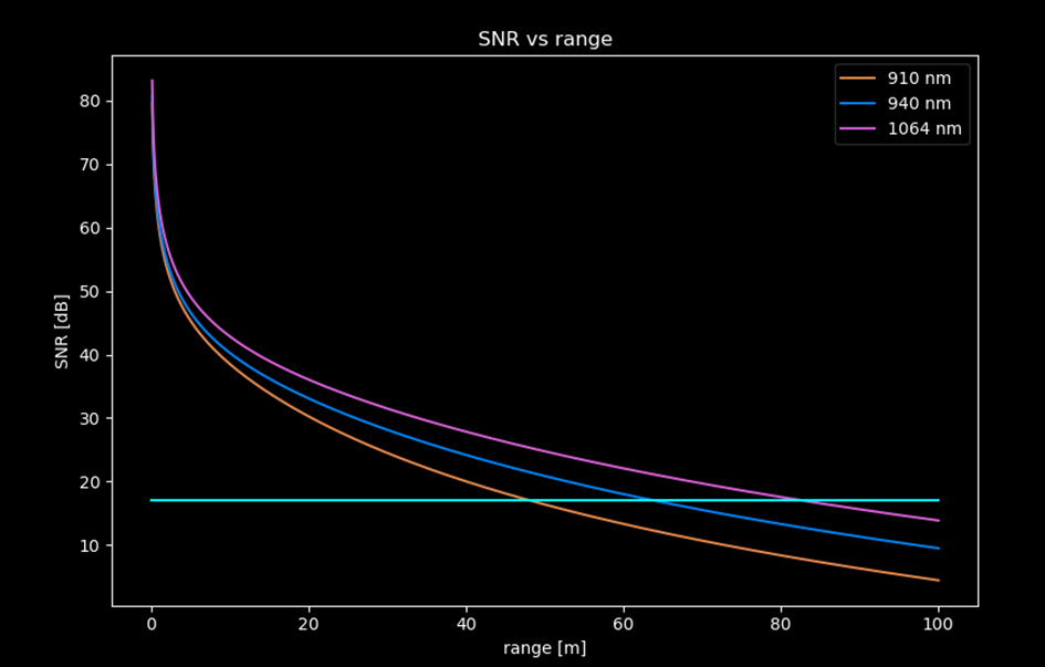
Fig 3. SNR versus range for three different wavelengths. The red line shows the detection threshold, which can be considered approximate (but not too far from the truth). In an actual linkbudget, one needs to add the contribution of detectors and the other electronics.

References

• McMahanon, Paul. LiDAR Technologies and Systems, SPIE Press Bellingham Washington. pp 97-98.