
The Perfect LiDAR – does it exist?
By Olov von Hofsten |
As a consultant, I have often been approached by unrealistic requirements from customers, and the LiDAR business is particularly prone to this. Perhaps because the technology is new. A customer often wants:
- Large field-of-view
- Long range
- High resolution
- Small form factor
- Low price
- Off-the-shelf (or ready in 2-3 weeks)
- Eye safety
If a customer was to write a specification for a camera system, this would not happen, as there are known and better understood trade-offs, for example between a large field-of-view and high resolution. My impression is that this is not yet the case in the LiDAR industry. One example is the trade-off between range and field-of-view. A scanning LiDAR system does not necessarily have this problem (which could be part of it), but mechanical scanning systems are becoming, to be honest, old news (at least for automotive LiDAR). Reliability and manufacturing yields are too big issues. For a true solid-state LiDAR with a lens and a detector array, the range will depend on the lens entrance pupil – this is what collects light. And this needs to have a certain size to achieve a certain required range. This is well known in Radar where range ~ √A [1] (A being the antenna area).
This is why a miniaturized long-range LiDAR is so difficult. Even if you make the electronics and detector small, you will still need an optical system with a large (5-15 mm?) entrance pupil. It doesn’t matter if you are using FMCW (a type of coherent LiDAR – see my previous blogpost on LiDAR detection techniques) or not, you simply need the photons.
Adding a large field-of-view (FOV) to this makes it even more difficult. A large field of view requires a short focal length (a strong lens), and a short focal length means a smaller aperture – you cannot have both. To understand why, it helps if you understand some fundamentals about optics.
You may have heard of etendue. It is used in illumination optics design. It states that the product of the range of positions (area) and the range of angles will not decrease, for a lossless system. This is also known as “You cannot make a laser out of a flashlight” or “You cannot focus the sun into an infinitely small point”. Quite intuitive and reasonable and it is one of the most important concepts in non-imaging optics and something that an optical designer faces in almost every project.
In imaging optics, the term etendue is not used. Instead it is called the “Lagrange Invariant” or the “Abbe Sine condition”. They have slightly different definitions: the Lagrange Invariant is only valid for a paraxial system and the Abbe sine condition uses sin(angle) which makes it applicable to higher angles. But the concept is the same, the product of angles and positions will remain constant (note: constant) in the absence of losses and aberrations.
Let us compare the detector plane and the entrance pupil plane. Let the size of the detector and the size of the entrance pupil be constants. The angular range at the detector is given by the F#, which is not realistically smaller than 1.2. This corresponds to an angle of arctan(1/(2*1.2)) = 0.4 radians. This is not a small angle so we need to use the Abbe sine condition.
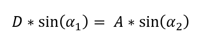
The field-of-view will be given by α2, A is the diameter of the entrance pupil and D is the width of the sensor. Replacing α2 by FOV and α1 by the F# equation derived earlier, we arrive at
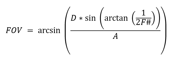
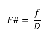
The focal length, f, is related to the F# and the entrance pupil diameter as
Let’s say the link budget (the budget on how many photons are needed for a specific detection) requires a 5 mm entrance pupil and the sensor size is 10 mm: this means that you have a maximum field-of-view of 100 degrees. Fig 1 shows a plot of FOV vs aperture for a 10 mm sensor.
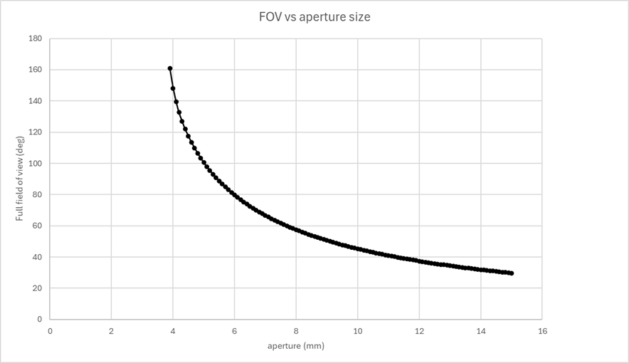
Figure 1. FOV vs aperture size for a 10 mm sensor and F# 1.2.
This is valid for systems without spherical aberration or coma (obviously not wanted). Also, this is valid for a system without distortion. With distortion, magnification changes with FOV and thereby also the entrance pupil. For example, by reducing the entrance pupil at higher angles, the range of angles can be increased. For example, 100% distortion (50 o to 100o) horizontally will give a 50% reduction in pupil area (corresponds to a pupil diameter reduction by 50% in one direction). Since range scales with the square root of the area, the range is reduced by √0.5 = 0.7, i.e 30% shorter range (in most cases). Anyway, most non-scanning LiDARs have roll-off of range for high angles, although it is not usually specified. An example of distortion and range roll-off is shown in figure 2.
To finish off the list I started with, the system form factor will depend on cost (number of aspheres or diffractives), resolution (number of surfaces in the system), sensor size (sets the lens diameter and limits FOV!), F# and how good your designer is. Let me know if you need help in finding someone really good 😊! Delivery time is never three weeks! Be realistic!
Furthermore, do not forget eye safety! This may limit your form factor, range or other key performance factors and is best to consider early in your design process.
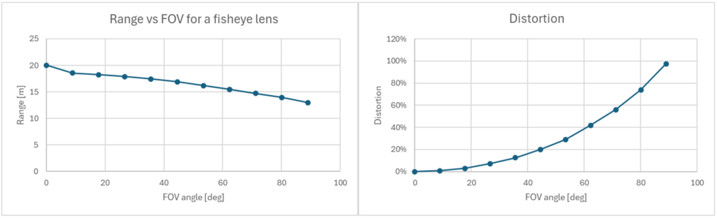
Figure 2. Roll off for an f-theta lens (fisheye), following the distortion (right graph)
References
[1] The Radar Range Equation, https://www.radartutorial.eu/01.basics/The%20Radar%20Range%20Equation.en.html