Understanding Camera Sharpness: The relationship between pixel count and resolution in smartphone cameras
By Jan Lüttgens |
In a previous post, we explained how sharpness and resolution are two separate characteristics of a camera system. Yet, from a consumer perspective they may seem to be somewhat correlated, as lens and image sensor resolution are matched and combined with a finely tuned image processing pipeline to yield optimal performance. For smartphone cameras and their form factor constraints, this meant more pixels equal higher resolution.
Indeed, there has been a relentless race towards smaller and smaller pixel sizes in CMOS image sensors used in smartphone cameras. A development that in some sense was driven more by a consumer misconception than a technical necessity. Main drawbacks of smaller pixels are higher noise and lower dynamic range. Regardless, pixel size decreased from around 6 µm in 2002 to 1 µm in 2010 (based on a relatively constant sensor size but increasing number of pixels). But around 2012 this development ran into an inevitable problem: the diffraction limit.
Even for an ideal, aberration-free lens, the smallest shape a point at infinity can be imaged to, is the diffraction pattern of its aperture, i.e. the smallest feature a lens can resolve. In the case of a circular aperture the resulting pattern is referred to as Airy pattern. The central area of the pattern contains about 84% of its energy and is called Airy disk.
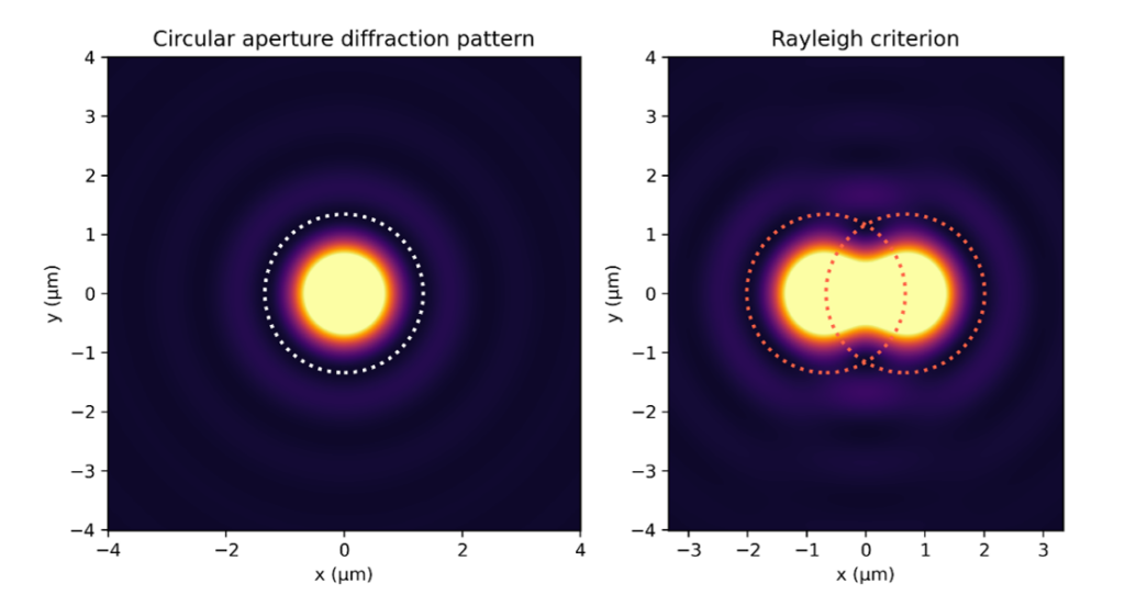
Figure 1. Left: Airy pattern calculated for an F/2 lens and green light (550 nm). The color map is scaled to show the side bands of the Airy pattern. The dashed line indicates the first minimum. Right: Closest distance 2 points can be resolved according to the Rayleigh criterion.
The Airy disk radius is defined by the first zero intercept of the Bessel function and depends on the lens F number N and the wavelength λ:
rairy = 1.22λN
This expression can be used to define a resolution criterion for digital cameras: The closest two Airy disks can approach each other while still being resolvable is the Airy disk radius, i.e., the maximum of one Airy disk falls onto the first minimum of the neighboring disk (Rayleigh criterion). For example, the Airy disk radius of an F/2 lens for green light (550 nm) is about 1.3 µm.
In 2011, Sony commercialized mobile phone image sensors with a 1.12 µm pixel size. For this pixel size an ideal F/2 lens would provide lower resolution, than the sensor can offer. And indeed, mobile phone lenses around this time were already diffraction limited, so in some sense, as sharp as they could possibly be.
However, today’s flagship smartphones come with up to 108 MP sensors down to sub-micron pixel sizes and sensor manufacturers continue to develop sensors with smaller pixel sizes (e.g. OmniVision and Samsung with 0.56 µm sensors and Sony with a 0.7 µm sensor in 2022). What is the reason behind this trend? To understand this, we need to have a look at modern image sensor layouts. To obtain a color image from an image sensor, on top of the spatial information, the sensor must store some information on the wavelength of light arriving at different image points. Afterall, humans have color vision because they have three dedicated cone-cell receptors on their retina that are sensitive to different bands of the electromagnetic spectrum. The most common way to achieve something similar for an image sensor is to equip the broadband-sensitive silicon pixels in CMOS sensors with bandpass filters. These only allow certain wavelength bands of light to reach the photosensitive area of the pixel. To create a color image, those filters must be arranged in some spatial pattern or color filter array (CFA) across the image sensor. The most common CFA pattern found on color image sensors is called the Bayer pattern, which contains one red, two green and one blue filter for a 2×2 pixel area (Figure 2).
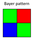
Figure 2. Illustration of a Bayer filter array
The filter ratios mimic approximately the ratio of color receptors on the human retina. This smallest repeatable unit (unit cell) is then repeated across the whole image sensor. With this arrangement, a scene is effectively captured in three colors and the image information is then processed to yield RGB color images which are widely supported by most LCD/OLED or modern displaying devices.
Capturing an image RGB image like this is illustrated in Figure 3, top row: A slanted edge is sampled by a monochrome and an RGB sensor with a Bayer CFA. However, extracting color information like this comes with a loss of spatial information per channel compared to a monochrome sensor, Figure 3, bottom row.
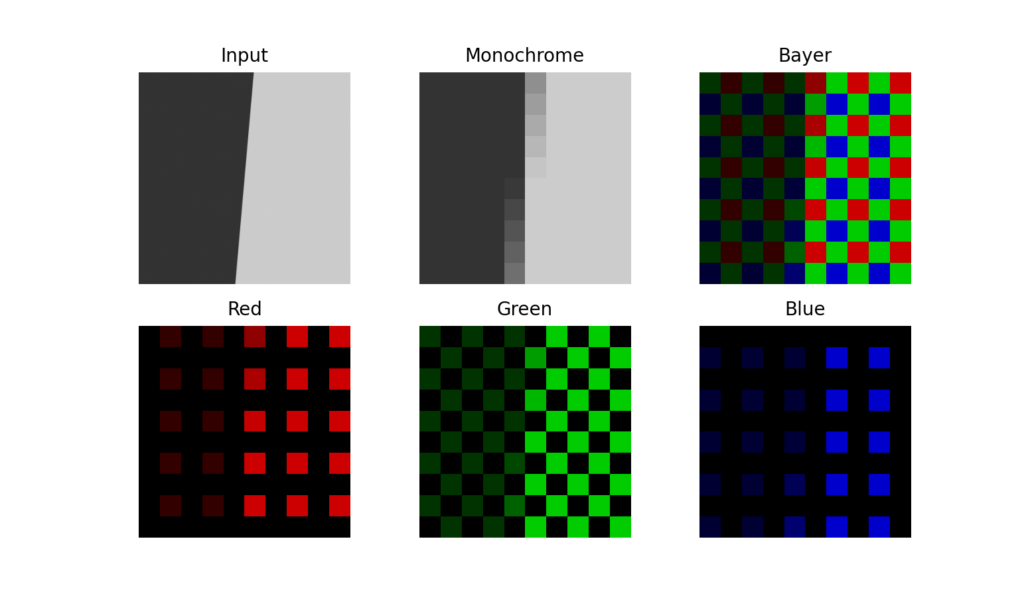
Figure 3. Top row: Slanted edge captured by a monochrome and a Bayer RGB sensor with same pixel pitch. Bottom row: Individual color channels for the Bayer RGB sensor.
Just considering the individual channels in Figure 3, you can convince yourself, that the spatial resolution of the red and blue channels is reduced by half. The resolution of the denser green channel is approximately reduced by √2. To illustrate this point, I sampled a resolution test chart (Siemens star) with a monochrome sensor and the Bayer RGB channels (Figure 4). The test chart consists of black wedges that get thinner and thinner towards the center. When the distance between the wedges approaches the pixel or sampling pitch of the sensor, swirly patterns occur due to aliasing. Even the dense green RGB channel shows considerably more aliasing than the monochrome sensor.
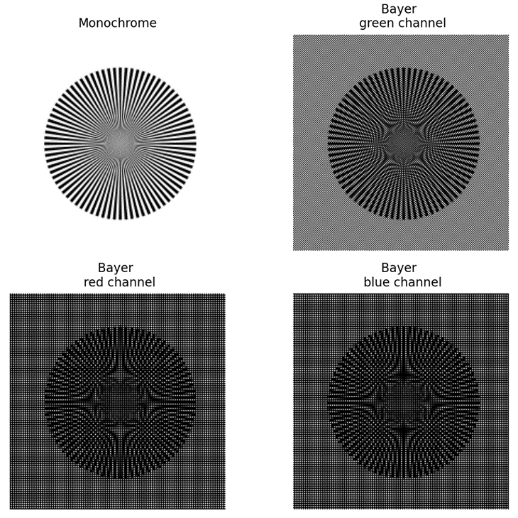
Figure 4. Resolution test chart (Siemens star) sampled by a monochrome sensor and by individual color channels of a Bayer RGB sensor. All channels are shown in grayscale for comparison.
Of course, the pictures on your smart phone do not look like the Bayer RGB image in Figure 3. The color channels are processed by interpolating the missing color information in each RGB channel to create a colored image. This is called demosaicing. But even smart demosaicing algorithms will struggle to reconstruct the missing spatial information compared to a monochrome image depending on the subject. This is illustrated in Figure 5. In the top row you see the slanted edge from Figure 3, but now sampled with higher resolution (500 × 500 pixels). The monochrome image (left) is next to indistinguishable from the interpolated RGB image (right). In the bottom row you see the Siemens star from Figure 4. For this more challenging test chart the interpolation algorithm fails to recover the spatial information one could have captured with a monochrome sensor. You can see this from the colored artifacts in the center of the interpolated RGB image (Figure 5 bottom row, right).
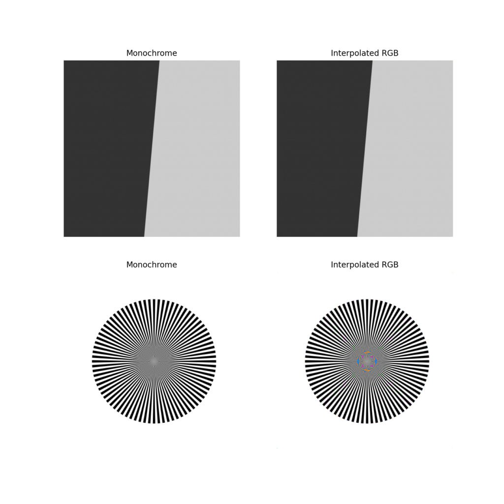
Figure 5. Monochrome sensor vs. interpolated RGB sensor.
Now that we understand the diffraction limit and image retrieval from an RGB sensor layout, let’s have a look at a popular smartphone that is specifically advertised for its imaging capability. The marketing material states that one of the cameras has an F/3 lens and a 48 MP sensor. The sensor is likely to have a 0.7 µm pixel size. But the Airy disk radius for green light (the light that we mostly rely on for spatial information in a Bayer sensor) is 2 µm! It looks like the pixel size is about 2.8 times smaller than the minimum resolvable feature for this F/3 lens.
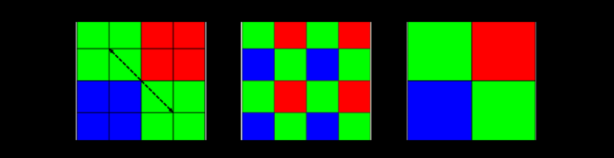
Under closer inspection of the sensor specification, we find that a so-called tetrapixel technology is used. This is a special variation of the Bayer pattern, where the smallest repeatable unit of the color filter array has 16 instead of 4 pixels as depicted in Figure 6, left. Depending on the manufacturer, this CFA may also be referred to as Tetracell, Quad Bayer, or 4-cell.
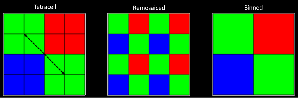
Figure 6. Left: Tetracell array with highest detectable frequency indicated. Center: Remosaiced Tetracell. Right: Binned Tetracell.
If we calculate the distance between the green tetra cells √2*2*0.7 µm, the smallest pitch the green subarray can detect is around 2 µm, which matches exactly the Airy disk radius of an F/3 lens. Thus, the √2*2 factor explains the mismatch of 2.8 between the Airy disk radius and the native pixel pitch of the sensor. So, the lens resolution matches the pitch of the green CFA cells, not the pixel pitch. Does this mean we can only get 12 MP image out of a 48 MP sensor?
Yes and no, the camera effectively captures the spatial information for the binned sensor shown in Figure 6, right. Using so-called remosaic algorithms it is possible to re-construct full resolution images, Figure 6, center, from the diffraction limited signal. Remosaicing algorithms are related to the demosaicing concept mentioned before. The information of the remosaiced image is a mathematical best-guess based on the diffraction limited image. The results can look quite convincing, but it is important to remember that the spatial information is synthetic (remember Figure 5). The caveat is that the remosaicing-functionality, in practice, is only used for bright scenes due to noise limitations. In low light, where noise becomes increasingly dominant, the signal of four pixels is binned to output an image with one-fourth the sensor resolution.
The true value of the Tetrapixel technology lies in the additional functionality it can support. Having more pixels available allows to repurpose individual pixels for tasks like autofocusing or HDR. For example, so-called dual gain HDR is supported by sensors, in which a subset of pixels captures an image at different gains, offering high-framerate HDR capability. Binning the tetrapixels allows to operate the sensor with reduced noise and increased dynamic range depending on the captured scene. Recent sensor developments target further improvements of these functionalities.
Having more pixels on your sensor may mean faster HDR or more reliable autofocus, but not necessarily higher resolution. Especially when it comes to smart phones, the number of sensor pixels alone does not tell you much about the resolution without considering the optics and image processing.
Read more about Eclipse knowledge in camera technology here: