Sharpness and resolution, part II

By Henrik Eliasson |

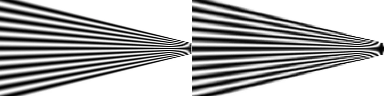
In the previous post we looked at the relation between optical resolution and sharpness. We could see that there is no clear correlation between the two. In this post we will complicate things a little by including the pixel resolution (we therefore assume a digital camera) into the mix. The last figure in the previous post is shown again in Figure 1.

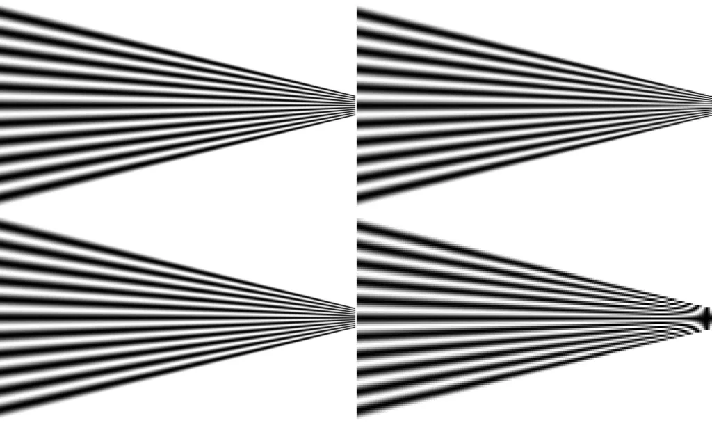
Here, the same target is shown at four different pixel resolutions, where the resolution is decreasing going from the top left through top right down to bottom right. As can be seen, the perceived sharpness is about the same in all cases. However, at the lower resolutions some other patterns start to appear at the highest spatial frequencies. This is an example of aliasing. It is called aliasing since a signal of a certain spatial frequency is taking on the appearance, i.e., an alias, of another spatial frequency. To understand what is going on, we need to analyze the spatial frequency content of the signal.

Recall the discussion about MTF from the previous post. The MTF tells us how much of a signal with a given spatial frequency is attenuated (or amplified) when propagated through the system. The spatial frequency spectrumdescribes the amplitude of the signal for a specific spatial frequency. When this signal is recorded by a digital system, it is sampled. This means that only specific instances of the signal are recorded. A simple example for a signal including only one spatial frequency is shown in Figure 2.

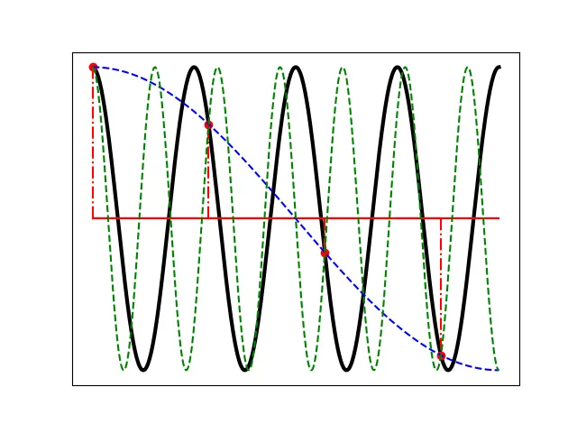
In the figure, we see that when reconstructing the continuous signal in black from the samples in red, ambiguity arises. Both the green and blue curves are possible continuous representations of the sampled signal. That is, they are aliases of the black signal. In fact, a sampled signal can have an infinite number of aliases. Which alias that is actually being reconstructed depends on the bandwidth of the system generating the signal as well as the sampling frequency. In Figure 3, the spatial frequency spectra of two signals, one exhibiting aliasing, and one that doesn’t, are shown. As is well known, an arbitrarily complex signal is composed of an infinite number of sinusoids at continuously increasing frequencies. The spatial frequency spectrum thus shows the amplitude of sinusoids associated with a particular spatial frequency. In this case, the unit on the horizontal axis is cycles per pixel, i.e., at the sampling frequency, one period is equal to the pixel pitch. For other applications, alternative units, such as cycles per millimeter, may be more appropriate.

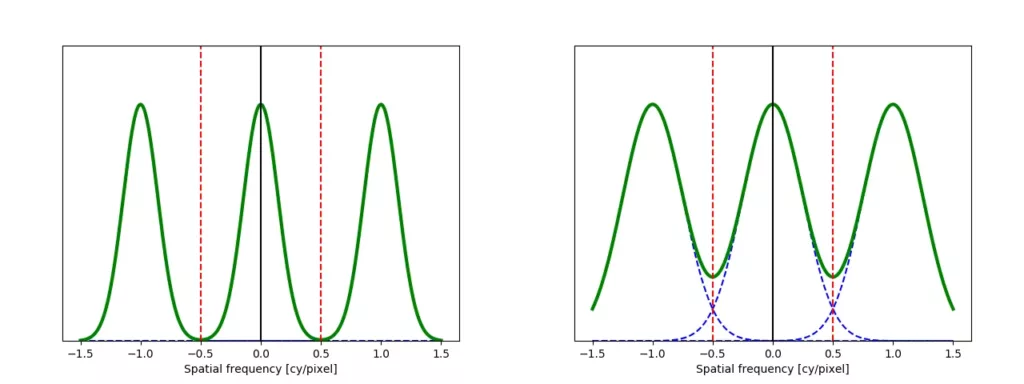
When sampling a signal, it can be shown mathematically that the spatial frequency spectrum will be affected by becoming repeated an infinite number of times at a period of the sampling frequency. Note that the spatial frequency spectrum also extends to negative frequencies and is mirrored around a spatial frequency of zero while the copies are mirrored around multiples of the sampling frequency at 1 cycle per pixel. As seen from the figure, if the bandwidth of the sampled signal extends beyond half the sampling frequency, the signal from the higher-order copies will leak into the zeroth order spectrum. This causes aliasing since higher spatial frequencies consequently will be “folded” back into the lowest order spectrum. Going back to the discussion, we can now see that the particular alias that will be reconstructed depends on which of the higher order spectra is leaking into the lowest order spectrum.

We now also see how we can avoid aliasing: make sure that the bandwidth of the signal does not extend beyond half the sampling frequency, known as the Nyquist frequency. To do this, we can apply a filter to the signal that removes signal above the Nyquist frequency before sampling. In case of a camera, the lens will act as such a filter. The MTF describes how signals at different spatial frequencies are attenuated and therefore constitutes a description of the spatial filtering characteristics of the lens. Thus, when designing a lens for a camera, the aim should be to produce an MTF with as high values as possible for spatial frequencies below the Nyquist frequency and zero above it. In practice, this is (as so often is the case) harder than it sounds. This results in a compromise between avoiding aliasing and maintaining sharpness as much as possible.

The images in Figure 1show no significant difference in sharpness depending on pixel resolution. From the discussion above, we now realize that, in a well-designed lens and camera combination, there will indeed be a relation between sharpness and pixel resolution, but in an indirect way. If we want to avoid aliasing artifacts at higher spatial frequencies, the sharpness will generally be affected. Thus, a 2-megapixel camera will generally have lower sharpness than an 8 megapixel camera.

An antialiasing filter is sometimes used in order to mitigate the effects of aliasing. However, such a filter will also to some extent reduce sharpness. As image sensor resolutions have increased, such filters have become less common, since higher resolutions make such filters less needed. Furthermore, by using a higher pixel resolution than actually needed (i.e., oversampling), it is possible to obtain an image at the desired resolution with higher sharpness by using efficient digital filters.

The discussion in this post has been restricted to monochrome cameras. For a color camera, things become even more complicated. This will be the subject of the next post in this series.