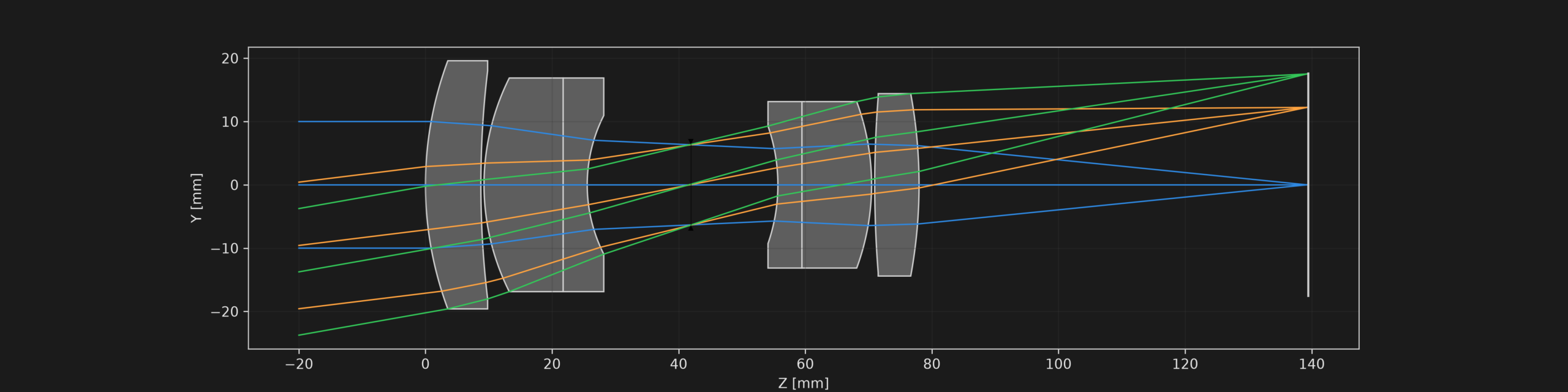
Optiland – Can you use an open-source tool for optical design?

By Madeleine Åkeson|

Have you ever wanted to make, analyze or adjust an optical design, but did not have access to a license for an optical design software such as Zemax?
Or, have you ever wanted to compare analyses from different lens designs without risking accidentally changing something in the actual design?
Or maybe you have just wished that you could more easily control the design and the analysis – create your own type of surface, make your own merit function operands, or write your own functions to set and analyze the parameters you are particularly interested in?

If so, you might be interested in Optiland.

What is Optiland?

Optiland is an open-source Python library for optical design, analysis, and optimization. This means, it is free to use and the code is open to read and modify. It can also be combined with other Python libraries, as well as with functionalities added by the user, by simply writing your own functions and classes.

You can think of it as a sequential Zemax which you can more easily modify to your liking (unfortunately non-sequential mode is not yet implemented).

What can Optiland do?

Optiland supports a wide range of capabilities including:

• Designing systems with standard surfaces (spherical, aspherical, paraxial, …) as well as possibility to define your own surface types
• Visualizing systems in 2D/3D, tracing rays, and performing analyses (MTF, PSF, etc)
• Optimization and tolerance analysis. The optimization support includes a variety of algorithms and differentiable ray tracing.
• Importing and exporting design files compatible with other software such as Zemax, Code V and Oslo

Getting started with Optiland

You can install Optiland to your Python environment by simply typing

pip install optiland

Creating a simple lens system is straightforward and the code is mostly self-explanatory:

from optiland import optic
import numpy as np
lens = optic.Optic()
# add surfaces
lens.surfaces.add(index=0, thickness=np.inf)
lens.surfaces.add(index=1, thickness=5, radius=100, is_stop=True, material="N-SF11")
lens.surfaces.add(index=2, thickness=112, radius=-1000)
lens.surfaces.add(index=3)
# add aperture
lens.set_aperture(aperture_type="EPD", value=25)
# add fields
lens.fields.set_type(field_type="angle")
lens.fields.add(y=0.0)
lens.fields.add(y=0.7)
lens.fields.add(y=1.0)
# add wavelengths
lens.wavelengths.add(value=0.44)
lens.wavelengths.add(value=0.55, is_primary=True)
lens.wavelengths.add(value=0.66)

# show system info and layout
lens.draw()
lens.info()

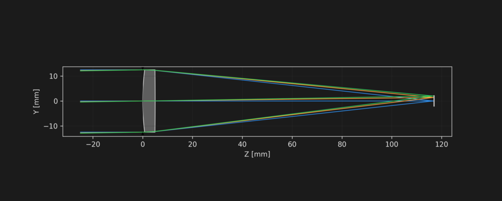
The result (layout by lens.draw() and tabular info by lens.info()) is shown in the figure below. In short, to create your design you set up the surfaces of the system, and the system info (aperture, wavelength, fields), and you can do this in whatever order you feel like. From here, you can add more surfaces, optimize the system, and perform analysis as well as check tolerances.

Of course you can also load surface parameters from a file, calculate them using NumPy or write any functions that suit your system, or just load the entire design for analysis.

For analysis, the basic tools you would expect are available, such as aberration data, spot diagram, PSF and MTF plots, etc.

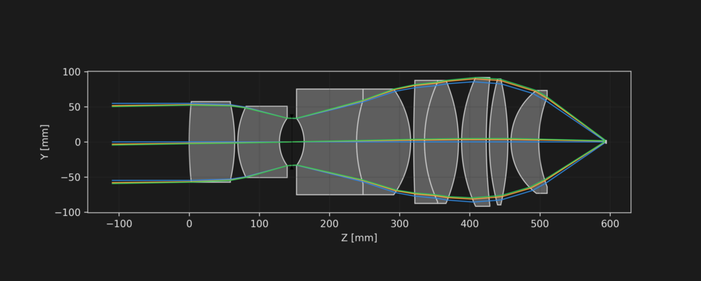
One thing that I appreciate is how easy it is to plot different ray properties throughout the system. For example, consider this microscope objective (loaded from optiland.samples.Objective60x) and the corresponding spot diagrams for three field points:

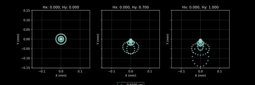
Looking at the previous figure, I get curious to know more about the shape of the (0, 1) field spot diagram. To investigate this further using Optiland, I can simply perform a ray trace, and then color the spot diagram by different properties. In the code example below, I choose to visualize this by coloring the spot diagram based on

• optical path difference (OPD)
• image plane incidence angle (in this case simply calculated from Z direction cosine since the image surface is flat and the traced rays only have y and z components)
• radial position of rays at stop surface

Here is a code snippet showing how to do this (most of the plotting code omitted):

lens.trace(Hx=0, Hy=1, wavelength=0.615, num_rays=15, distribution="hexapolar")
num_surfaces = lens.surfaces.num_surfaces
opd = lens.surfaces.opd[num_surfaces - 1, :]
N = lens.surfaces.N[num_surfaces - 1, :]
theta_inc = np.rad2deg(np.arccos(N))
x_stop = lens.surfaces.x[lens.surfaces.stop_index, :]
y_stop = lens.surfaces.y[lens.surfaces.stop_index, :]
r_stop = np.sqrt(x_stop**2 + y_stop**2)
x_image = lens.surfaces.x[num_surfaces - 1, :]
y_image = lens.surfaces.y[num_surfaces - 1, :]

plt.figure() 
plt.subplot(1,3,1)
plt.scatter(x_image, y_image, c=opd) 
...
plt.subplot(1,3,2)
plt.scatter(x_image, y_image, c=theta_inc) 
...
plt.subplot(1,3,3)
plt.scatter(x_image, y_image, c=r_stop) 
...

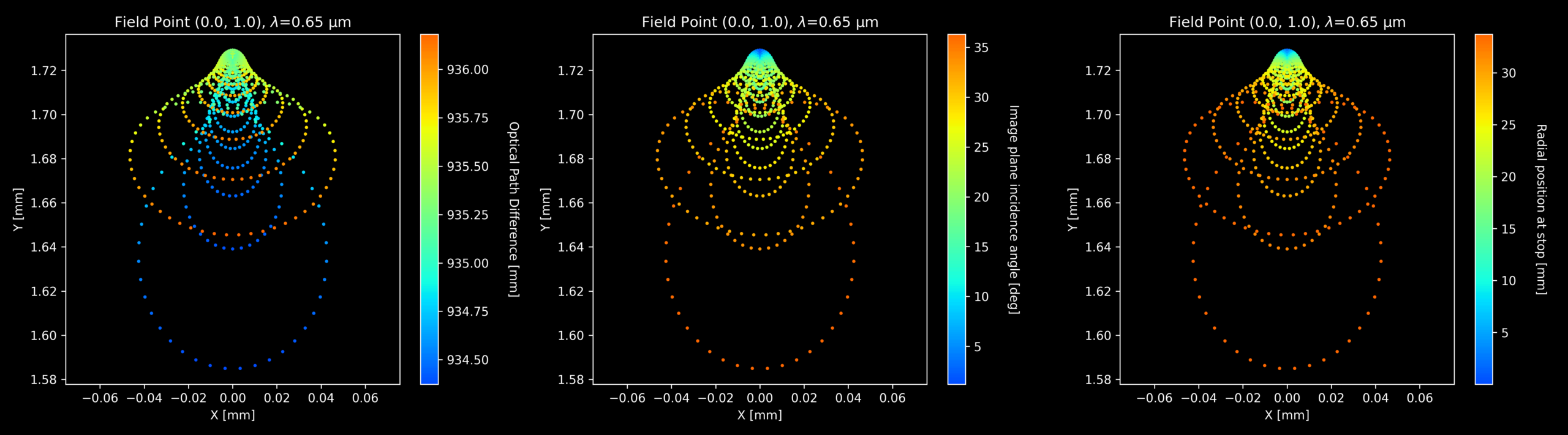
From these plots, it is easy to see approximately which parts of the stop and which incidence angles contribute to the shape of the spot diagram, and the corresponding OPD. I appreciate getting visual information like this, and from this point on, I could continue the analysis by drawing specific rays, maybe examine the effect of decreasing the stop size, or reoptimize the lens.

How to separate optical design from analysis

When I work with designing a system, in the process of finding the best solution, I often have several systems which I want to compare. But opening them up one by one in Zemax to set up the same analysis takes time, and also generally leaves me a little uncertain. Did I really set up the same sampling for all these MTFs or is one of them different? Does one analysis look better because I only included one wavelength, where I should have included all? And do I really have all results grouped with the correct parameters, or have I mixed something up?

One solution to this is to just separate the design from the analysis and data extraction. In Optiland, I can load my design (made in Optiland, or Zemax, Code V or Oslo) and setup, and then save the results of the analysis I am interested in. Then, I just do the same for the next design candidate, using the same code, with no uncertainties whether the analysis uses the same parameters. I can do them all in a loop and automatically save results and plots, as well as system parameters, into files with proper naming and headings. And the design files themselves are unaltered. Convenient, right?

In the example below, I load two example objectives (Telephoto and DoubleGauss, both from samples.Objectives) and plot the MTF for a side by side comparison. To be sure that I compare the same data, I have written a function to remove any saved field points and wavelengths (remove_fields_and_wavelengths(lens)), and then I set my own parameters.

Here is a code snippet with the relevant code:

fields = [0, 7, 10]
wavelength = 0.55
lenses = [Telephoto(), DoubleGauss()]
for lens in lenses:
    remove_fields_and_wavelengths(lens)
    lens.fields.add(fields[0])
    lens.fields.add(fields[1])
    lens.fields.add(fields[2])
    lens.wavelengths.add(wavelength, is_primary=True)
    lens.draw()
    mtf = FFTMTF(lens, num_rays=128, max_freq=150)
    mtf.view()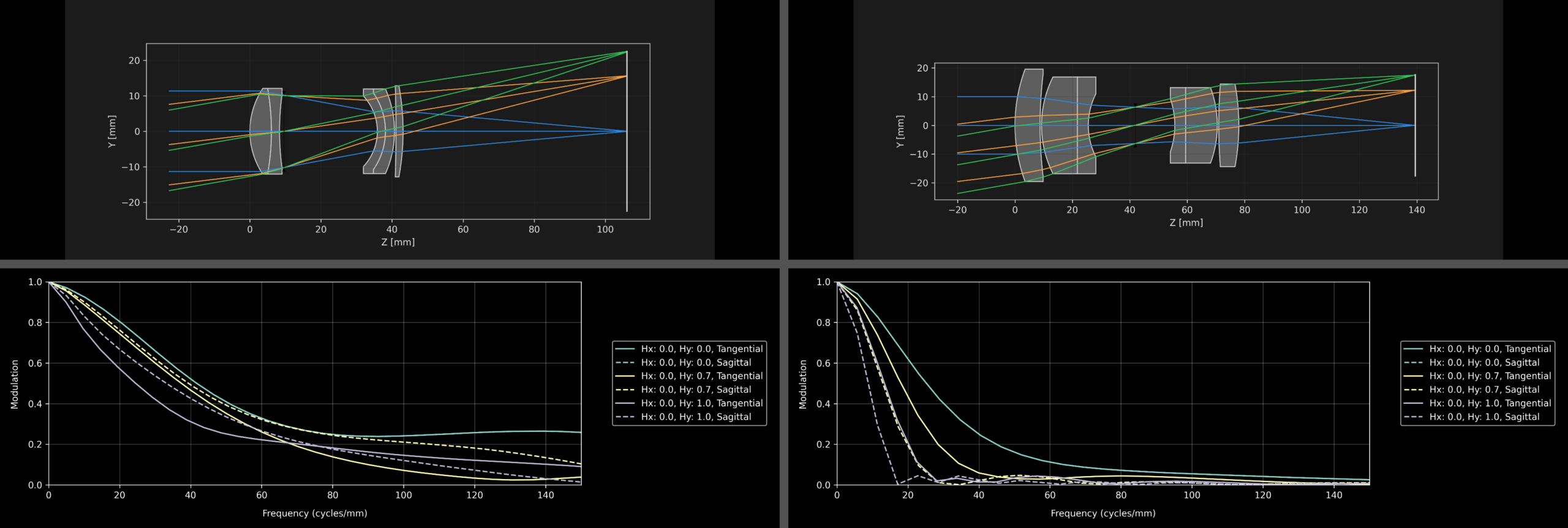

The result shown above is a side-by-side comparison of the performance of the two lenses, where I know that I have performed the exact same analysis, and the design files are unaltered. While this example compares the performance of two quite different lenses, it could of course instead have been comparing a few different outcomes from an optimization run, or results before and after adding an extra constraint to the optimization.

Challenges and drawbacks with Optiland

While promising, it is important to be aware of some challenges and drawbacks with Optiland:

• Optiland is still under active development. Some features are not tested exhaustively, and the code syntax is still evolving, which means that your old code may need to be updated when updating to a new version of Optiland. And some functions may not work as expected – it is still a good idea to compare the results from an analysis to what you get using another ray tracing software
• Various bugs are still found, but this is improving over time thanks to its open-source nature. I have noted and reported a few bugs, and found that the community is very responsive and helpful
• Compared to Zemax and other optic design software, some features are missing. Of course, non-sequential ray tracing is an important one, but also less critical features and functionalities are still to be implemented.

Possibilities ahead

This blog post only touches the surface of what is possible with Optiland. One of its strengths is being open-source, so that you can add functionality as you need it, and if you want to know exactly how something is done, you can simply read the source code. Also, feature requests and bug reports are handled promptly on GitHub, and contributions are of course welcome if you are up for it!

We at Eclipse Optics will continue to explore optical design and simulation software, so stay tuned for future blog posts focusing on the growing possibilities with Optiland. In our next post, we will explore how to use Zemax files in Optiland!

---

More info

For the code in this blog post, Optiland 0.6.0 has been used.
For more information, we recommend reading the documentation, and release notes at GitHub.